Section 2: Sonic Visualiser
Contents
Section 2: Sonic Visualiser
Download Sonic Visualiser software and extract it to your system.
Navigate to the download page for Sonic Visualiser linked here.
If you are using a Mac computer, click the download link for Mac on the right of the page. If you are using Windows, you will likely need to use the 64-bit installer, on the left of the page. If you experience problems with this (or are using an older system, for instance), you may need to use the 32-bit installer.
Note
The Windows version of Sonic Visualiser runs on most modern updates. The Mac version requires OSX 10.12 or later.
If you’re using a Mac and receive a warning along the lines of ‘application can’t be opened because Apple cannot check it for malicious software’, you will need to temporarily override your Mac security settings (don’t worry, the app is perfectly safe). First, go to Security & Privacy. Next, click the Open Anyway button in the General pane to confirm your intent to open or install the app. If this doesn’t work, you can also try dragging and dropping the download to your applications folder, and then right clicking on it to run. If none of these options work, please send me an email and I’ll see what I can do!
If you’re using an operating system that isn’t currently supported by Sonic Visualiser (e.g. a Chromebook) you can also access Sonic Visualiser on the computers in the CMS. For card access to the CMS, visit the website here and email Mustafa Beg.
Whatever version you are using, download the program using the primary link. Open up the .msi (Windows) or .dmg (Mac) file you downloaded and follow the installer through to the end to complete the installation. On Windows, you may need to wait a while before pressing ‘Yes’ when the User Account Control screen pops up.
Select ONE performance for further study, download audio and transcription files.
Browse to the OneDrive folder linked here, you should find a folder called ‘Audio Files’.
Inside this folder are six recordings of the exposition from the first movement of Beethoven’s 5th Symphony. All of these recordings were made within the last ten years, in contrast to the recordings from 1920-1990 considered by Bowen. Have a listen to these and download ONE of the performances that you want to work with in this exercise.
There is also a single .pdf file containing the score of the exposition. You should download this also.
Note
If you have time after completing an analysis of one recording, you are more than welcome to repeat the same process on another. Do your conclusions still hold up, or might one recording be an outlier?
Open the audio spectrogram in Sonic Visaliser.
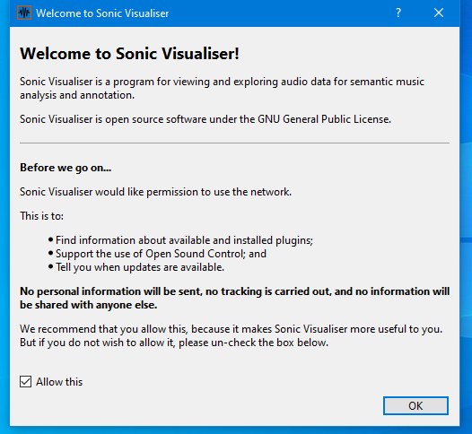
Open up Sonic Visualiser by locating it in the start menu (Windows) or Applications folder (Mac). You should be presented with the logo splash screen. The next thing you will see will be a welcome window that requests access to your internet network. Although we won’t be using any network features in this exercise, I’d recommend that you allow network access in case you want to use Sonic Visualiser in the future - it makes installing updates and plugins much easier.
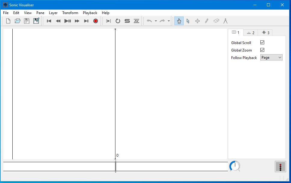
The next screen you should see is a blank Sonic Visualiser window:
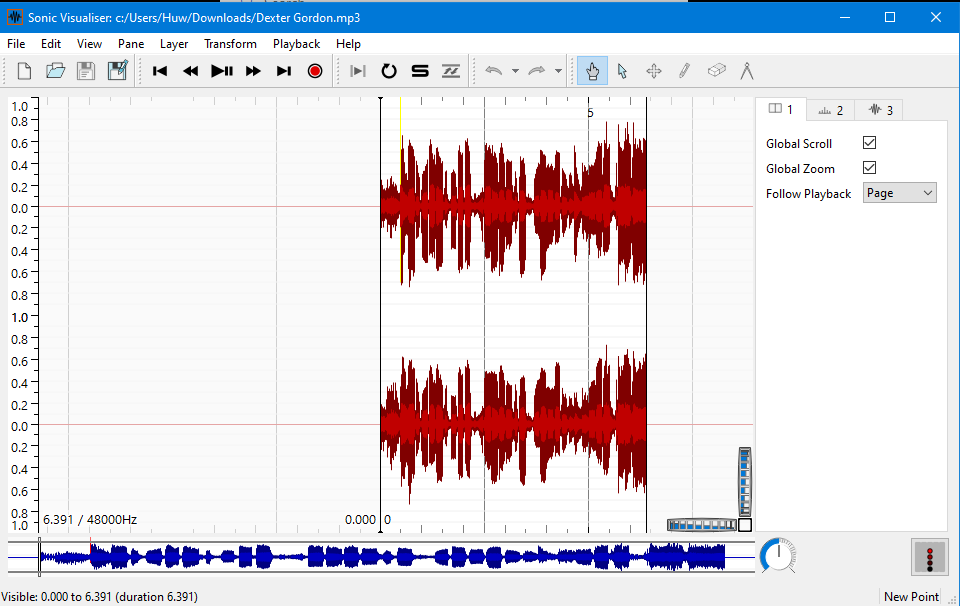
We now need to load in some audio. Open up the location where you saved the recording earlier in the file explorer (Windows) or finder (Mac), and drag and drop it onto the Sonic Visualiser window. You should see the waveform of the audio appear:
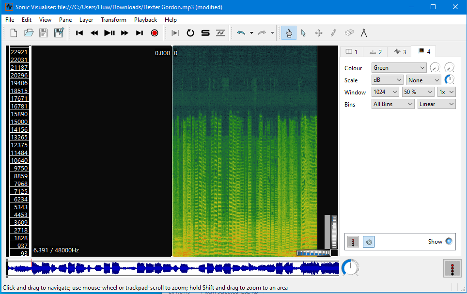
While interesting, this doesn’t help us much in locating the onset of individual bars or beats. A spectrogram is a better option, so click Layer at the top of the window, then Add Spectrogram and [NAME OF AUDIO].mp3: All Channels Mixed. This will shift to the Spectrogram view, where we can see the individual frequencies:
Note
The spectrogram view will default to green. For some people this might not be the best option, so you can choose the colour on the side panel. You can also adjust the threshold and colour rotation of the spectrogram using the two dials either side of the colour drop-down option, which may help when identifying note onsets. I find that the White on Black option with the threshold at approx -60dB and rotation -30 leads to good initial results.
We also need to be able to hear the recording in Sonic Visualiser. To do this, we can use the large transport buttons at the top of the window (next to the file open and save buttons), or press the spacebar.
Note
If you find that the playback is too fast, you can slow the recording down using the large dial in the bottom right of the screen (immediately to the right of the waveform).
Identify the duration of the exposition.
In our analysis, we need two key pieces of data to compare our modern recording to Bowen’s: the duration of the exposition in minutes and the average tempo of the second theme, in beats per minute. We’ll calculate the duration first.
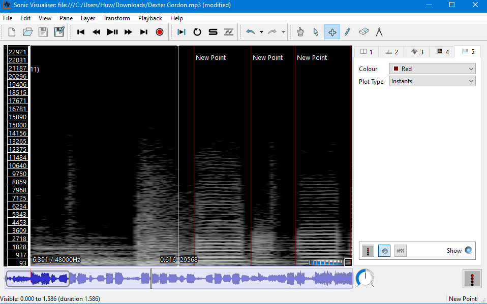
To do this, add a new time instants layer by clicking the Layer drop-down menu - Add New Time Instants Layer. You can now click anywhere on the spectrogram to add a point, which will be shown as a line across the spectrogram. To adjust the placement of a point, click the edit button at the top (next to the pencil and cursor icons) and drag the point to where you want it. You can also delete a point by clicking the eraser (next to the pencil and compass) then clicking on the point again.
Note
By default, Sonic Visualiser renders time instants as white lines. This can be confusing, as the playback line is also white. You can change the colour of the instants on the right-hand menu.
Once you’ve tried creating some time instant values, the next task is to place them at the start and end of the exposition. Open up the score and then, with the help of the spectrogram, place a time instant value onto the start and end of the exposition.
Note
Unfortunately for our purposes, the exposition starts with a quaver rest and ends with two bars of silence. To counteract this, treat the first sounding quaver (on the upbeat of beat 1) as the start and the repeat of this quaver as the end of the exposition.
Identify the BPM of the second theme.
Now that we’ve set time instants to mark the start and end of the exposition, we need to identify the beats per minute of the second theme, which Bowen claims to have gradually been speeding up since the 1930s and thus causing a decrease in duration of the exposition.
So that we don’t confuse our duration markings with our BPM markings when exporting the data, create a new time instants layer as we did before and make sure it is set to a different colour. As we did with the duration layer, place time instants onto the spectrogram in accordance with the score. We’re now interested in measuring the BPM, however, so you’ll need a new time instant for each crotchet beat.
Note
Although the second theme formally begins with the ‘horn call’ from bar 59, start measuring from when the violins bring the theme itself in in bar 63 - it’ll be easier to measure the crotchets here. For similar reasons, treat the fortissimo chord at bar 94 as the end of the second theme and stop counting beats from then.
Export your data for analysis.
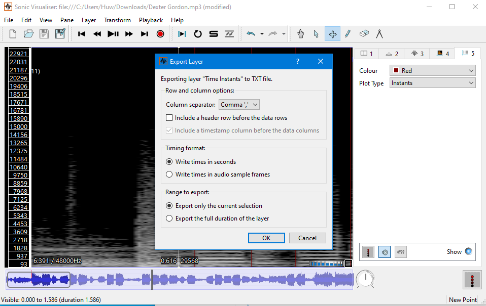
Once you’ve labelled all the onsets required to measure both the exposition duration and second theme BPM, it’s time to get the data out of Sonic Visualiser. Make sure your first time instants layer (for the duration) is active by selecting it in the panel on the right of the screen: it will likely be layer 5. Then, go to File - Export Annotation Layer. Choose where to save your file, select the file type .txt in the drop-down menu and press save.
Note
If you find that you get an error when trying to save, you may need to put .txt manually at the end of your filename - e.g. Timings.txt
In the ‘Export Layer’ dialogue window that follows, change the column seperator from Tabs (default) to Commas or Spaces: this will help us when we come to importing our data. Make sure that the timing format is in seconds and press OK to export.
Now, repeat these steps to generate a second .txt file for our BPM analysis. Make sure that your second time instants layer is selected from the panel on the right this time: it’ll probably be layer 6, unless you’ve added any others.
Now we’re ready to clean our data.